
Complete Guide of Dealing with Missing Data
Outline of this article
- Missing Data Mechanisms
- Simple missing data fixes: LVCF, mean imputation, dummy variable methods
- More complicated missing data fixes: Weighting, hotdecking, regression imputation
- Building blocks and overview of multiple imputation, including regresion imputation with noise
The way we handle missing data really depends on the missing data mechanisms. It has several cases such as missing completely at random, missing at random and not missing at random. Before that, we first need to go through some patterns that commonly appears as a problem in our dataset.
Examining Patterns of Missing Data
Missing data cases in a dataset:
These covers most common situations:
- Univariate Nonresponse:
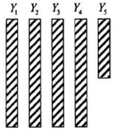
- Multivariate Two Patterns:
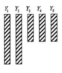
- Monotone:
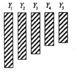
- General:

Notation and explanation Let R be the matrix of variables R1, R2,…,Rp, corresponding to variables in dataset, Y1, Y2, …,Yp, that indicate whether a given value of the corresponding Y variable is observed(=1) or missing(=0)
Missing Data Mechanisms:
In this part, we will need to analyze these three situtions before we come up with a solution to ignore/drop/compute missing data.
- Missing Completely at Random (MCAR)
- Missing at Random (MAR)
-
Missingness depends on observed values of the variables
- Not Missing at Random(NMAR), also called Missing Not at Random
) Missingness depends on the values of the items that are missing!
MCAR and MAR are both ignorable missing data mechanisms. The term ignorable reflects that fact that for these missing data mechanisms we can make inferences using our data without having to include a model for the missing data mechanism within our analysis model. NMAR is a non-ignorable missing data mechanism,
Simple missing data methods:
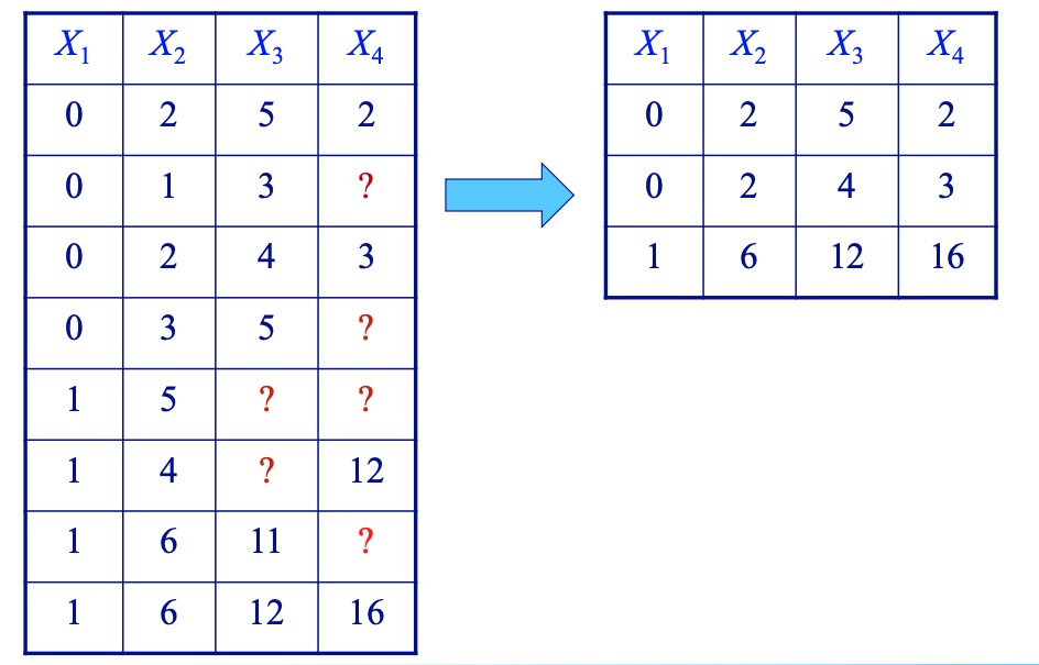
Once we figure out the missing data mechanism, we can decide to either drop or compute.
Methods that throw away data
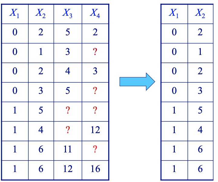
This is the easy part, two ways to do it- either drop the variable (the column) or just the observations (the row).
- Complete cases (listwise deletion)
- Complete variables (available case)
Methods that don’t throw away data
This method is commonly used in the current research field. This can keep some information that your data want to perserve and also don’t confuse people.
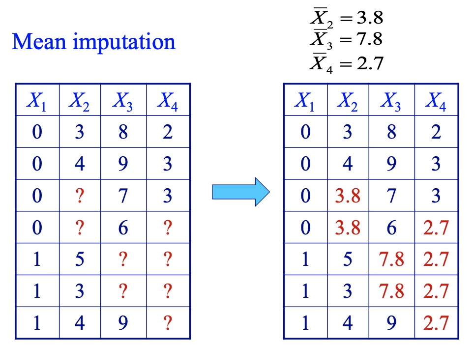
- Mean imputation
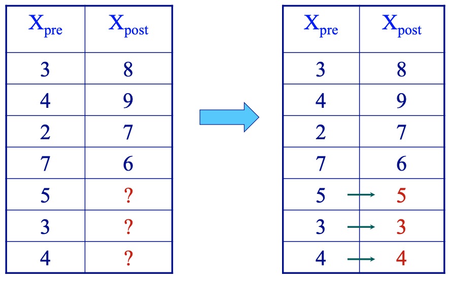
- Last value carried forward
- Dummy variable method
- For example, for each predictor variable with missing data, fills in missing values with 0 or the mean and then includes a new variable that is an indicator for missingness for the original variable with missing data.
- Reports from others
- For example, we are missing data regarding the fathers of children in a dataset, we can probably fill these values in with mother’s report of the values.
More complicated missing data methods
This is the hardest part, this method is relatively complicated but can cause less bias in your dataset for further estimation.
Methods that throw away data
- Non-response weighting
- Suppose only one variable has missing data, we can build a model to predict whether a vlaue is observed using observed values from the other variables. Then use these predicted probabilities to create survey weights of the form
to make the complete case sample representative of the full sample once again. Typically we normalize by multiplying the weights by the overall (marginal) probability of missingness, P(Ri. This way the weights will sum to the number of people left in the complete case sample.
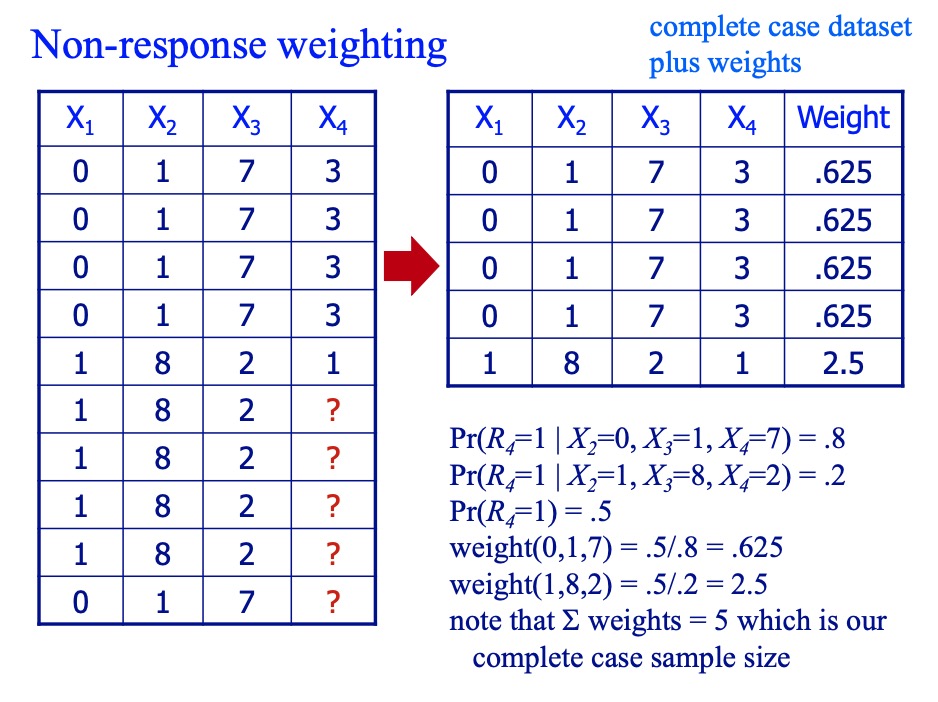
- Suppose only one variable has missing data, we can build a model to predict whether a vlaue is observed using observed values from the other variables. Then use these predicted probabilities to create survey weights of the form
Methods that don’t throw away data
- Hotdecking
- Replaces missing values using other values found in the dataset.For example, for each person with a missing value on variable Y, find another person who has all the same values (or close to the same values) on observed variables
, and use that person’s Y value.
- Replaces missing values using other values found in the dataset.For example, for each person with a missing value on variable Y, find another person who has all the same values (or close to the same values) on observed variables
- Regression imputation
- Suppose only one variable has missing data, within the complete case sample, build a model that predicts the values of that variable.
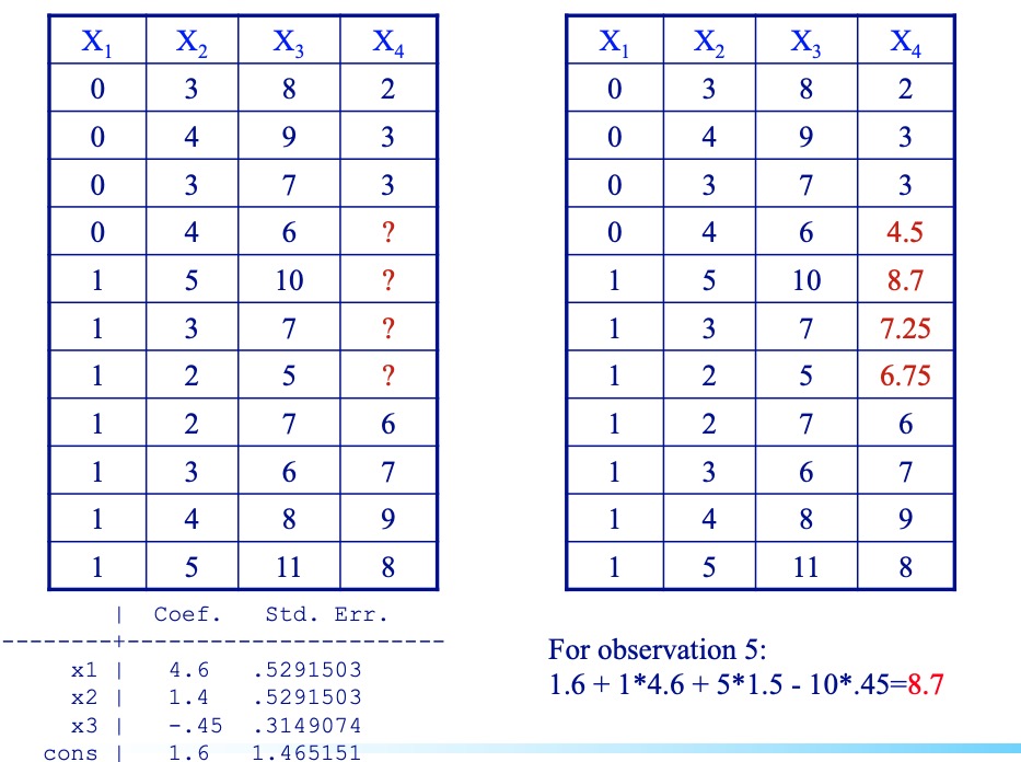
- Suppose only one variable has missing data, within the complete case sample, build a model that predicts the values of that variable.
Multiple regression imputation with noise
Multiple imputation uses observed data to impute missing values that reflect both sampling variability and model uncertainty. It creates several imputations for each missing value and thus creates several completed datasets.
However, it can be difficult to implement when there are complex patterns of missing data;
noise = rnorm(length(y.imp),0,summary(mod)$sigma))
y.imps = y.imp + noise
Stochastically impute for binary data:
mod =  glm(y~ pred1 + pred2, data = dat.cc, family = 'binomial')
ps = predict(mod, newdata= dat.dropped)
y.imps = rbinom(sum(Ry == 0 ), 1, ps)
Stochastically impute for unordered categoricals
library(nnet)
mmod = multinom(y ~ pred1 + pred2, data =  dat.cc)
ps = predict(mmod, type = 'prob', newdata = dat.dropped)
Assume ps is a matrix of probabilities obtained from fitted model combined with predictor data for observations you want to impute for
k = 5  # k is the number of categories
cat.imps = numeric(nimp)
# nimp is the number to be imputed (sum(Ry == 0))

for (i in 1: nimp) {
cat.imps[i] = sum(rmultinom(1,1,ps[i,]) * c(1:k))
}
The part within the parentheses will create a vector of 0’s except the one category where the draw occurred and that slot will now show its category number rather than a 1. So when you sum all you get back is that category number.
MI Strengths:
- Maintains entire dataset
- Uses all available information
- Weak (more plausible) assumptions about the missing data mechanism
- Properly reflects two kinds of uncertainty about the missing data (so, confidence intervals have correct coverage properties)
- Sampling uncertainty
- Model uncertainty
- Maintains relationships between variables
- One set of imputed datasets can be used for many analyses (allowing for release, for example, of public use imputed datasets)
MI Weaknesses:
- Can be more complex to implement (though with current software this is becoming less and less of an issue)
- Have to rely on modeling assumptions
How does it work?
- Specify a model for the complete data, and fit
- Use this model to predict missing values
- Repeat 1-2 M times to create M complete datasets
- Perform your desired analysis in each dataset
Implementation in R:
library(mi)
# load the data
data(nlsyV)
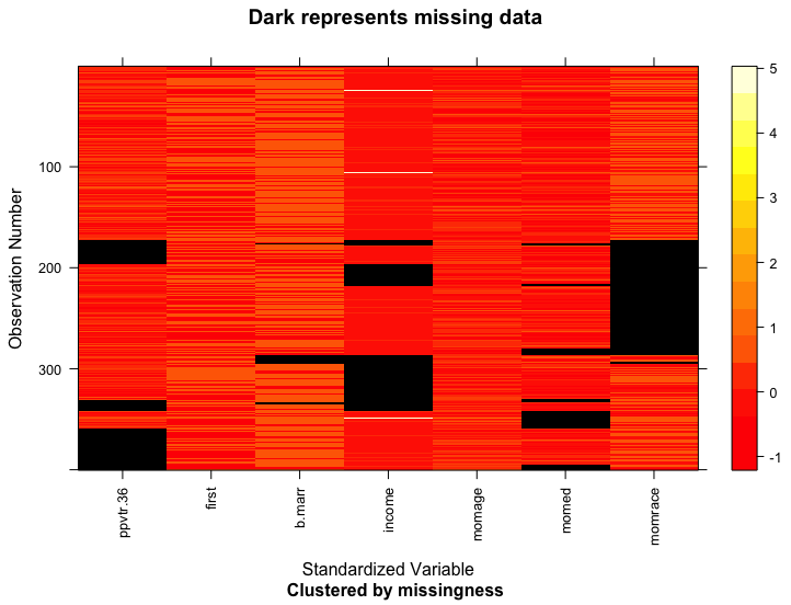
# Create a missing_data object, look at the data and the missing data pattern
mdf = missing_data.frame(nlsyV)
## NOTE: In the following pairs of variables, the missingness pattern of the first is a subset of the second.
##  Please verify whether they are in fact logically distinct variables.
##      [,1]     [,2]
## [1,] "b.marr" "income"
image(mdf)
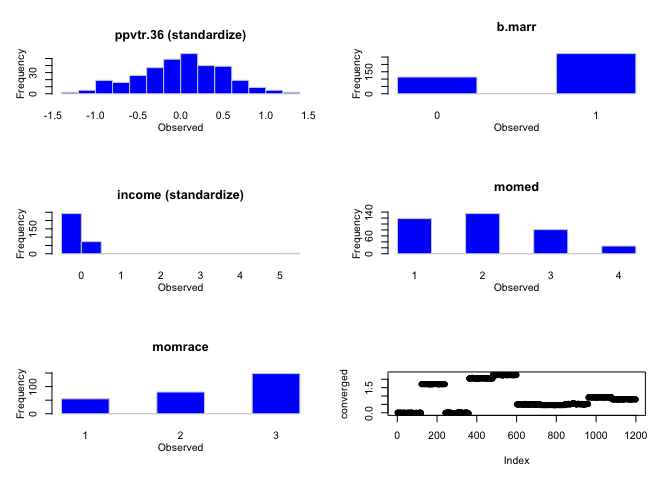
hist(mdf)
# Examine the default choices for imputation models
show(mdf)
## Object of class missing_data.frame with 400 observations on 7 variables
##
## There are 20 missing data patterns
##
## Append '@patterns' to this missing_data.frame to access the corresponding pattern for every observation or perhaps use table()
##
##                         type missing method  model
## ppvtr.36          continuous      75    ppd linear
## first                 binary       0   <NA>   <NA>
## b.marr                binary      12    ppd  logit
## income            continuous      82    ppd linear
## momage            continuous       0   <NA>   <NA>
## momed    ordered-categorical      40    ppd ologit
## momrace  ordered-categorical     117    ppd ologit
##
##               family     link transformation
## ppvtr.36    gaussian identity    standardize
## first           <NA>     <NA>           <NA>
## b.marr      binomial    logit           <NA>
## income      gaussian identity    standardize
## momage          <NA>     <NA>    standardize
## momed    multinomial    logit           <NA>
## momrace  multinomial    logit           <NA>
# Make changes to imputation models if necessary
mdf <- change(mdf, y = c('momed', 'momrace'), what = 'type', to = 'un') # changed ordered to unordered
show(mdf)
## Object of class missing_data.frame with 400 observations on 7 variables
##
## There are 20 missing data patterns
##
## Append '@patterns' to this missing_data.frame to access the corresponding pattern for every observation or perhaps use table()
##
##                           type missing method  model
## ppvtr.36            continuous      75    ppd linear
## first                   binary       0   <NA>   <NA>
## b.marr                  binary      12    ppd  logit
## income              continuous      82    ppd linear
## momage              continuous       0   <NA>   <NA>
## momed    unordered-categorical      40    ppd mlogit
## momrace  unordered-categorical     117    ppd mlogit
##
##               family     link transformation
## ppvtr.36    gaussian identity    standardize
## first           <NA>     <NA>           <NA>
## b.marr      binomial    logit           <NA>
## income      gaussian identity    standardize
## momage          <NA>     <NA>    standardize
## momed    multinomial    logit           <NA>
## momrace  multinomial    logit           <NA>
# Impute until converged
imputations <- mi(mdf)
converged <- mi2BUGS(imputations)
# Plot diagnostics
Rhats(imputations) # some values are greater than 1.1
## mean_ppvtr.36   mean_b.marr   mean_income    mean_momed  mean_momrace
##     0.9934971     1.1135680     1.4610195     1.0873550     1.0166828
##   sd_ppvtr.36     sd_b.marr     sd_income      sd_momed    sd_momrace
##     1.0089440     1.1148122     1.2526901     0.9943404     1.0490912
# Iterate bewtween step 4-6 if necessary
mdf2 <- change(mdf, y = 'income', what = 'type', to ='nonn')
imputations2 <- mi(mdf2, n.iter = 60)
Rhats(imputations2) # much better
## mean_ppvtr.36   mean_b.marr   mean_income    mean_momed  mean_momrace
##     1.0007753     1.0117282     1.0091317     0.9994462     1.0218410
##   sd_ppvtr.36     sd_b.marr     sd_income      sd_momed    sd_momrace
##     1.0023546     1.0118700     1.0130152     1.0154492     1.0287456
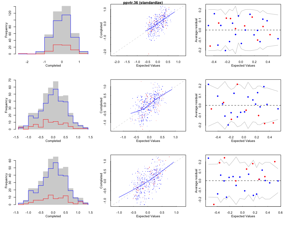
Visualize the computed missing values Red lines/dots are computed; blue lines/dots are observed;
# Run final pooled analysis
analysis <- pool(ppvtr.36 ~ first + b.marr + scale(income) + momage + momed + momrace, imputations2, m = 5)
print(analysis)
## bayesglm(formula = ppvtr.36 ~ first + b.marr + scale(income) +
##     momage + momed + momrace, data = imputations2, m = 5)
##               coef.est coef.se
## (Intercept)   73.91     7.86
## first1         3.91     2.02
## b.marr1        5.76     2.26
## scale(income)  0.57     0.92
## momage        -0.10     0.32
## momed2         4.46     2.35
## momed3         8.37     2.98
## momed4        15.01     4.75
## momrace2      -6.84     3.47
## momrace3      11.34     2.64
## n = 390, k = 10
## residual deviance = 96006.6, null deviance = 145237.1 (difference = 49230.6)
## overdispersion parameter = 246.2
## residual sd is sqrt(overdispersion) = 15.69
# Now compare to complete case analysis

glm(formula = ppvtr.36 ~ first+ b.marr+ scale(income) + momage + factor(momed) + factor(momrace), family = gaussian, data = nlsyV)
##
## Call:  glm(formula = ppvtr.36 ~ first + b.marr + scale(income) + momage +
##     factor(momed) + factor(momrace), family = gaussian, data = nlsyV)
##
## Coefficients:
##      (Intercept)             first            b.marr     scale(income)
##          64.9769            5.2662            6.1983            0.6214
##           momage    factor(momed)2    factor(momed)3    factor(momed)4
##           0.1778            4.2121            9.5115            7.4224
## factor(momrace)2  factor(momrace)3
##          -3.8900           14.1495
##
## Degrees of Freedom: 171 Total (i.e. Null);  162 Residual
##   (228 observations deleted due to missingness)
## Null Deviance:       63870
## Residual Deviance: 40100     AIC: 1448
Other R package such as ‘mice’ can do the mulitple imputation effectively as well. For more Gelman-Robin Rhat Statistics explanation, please refer to this paper here