Understand Central Limit Theorem from Simulation Data in Python

I have been asking about Central Limit Theorem frequently during interview. Seems like it’s easy, and we have been studing it since STAT101. But it’s relatively hard to explain it thoroughly. So I am going to illustrate it using interactive graph produced by Python Plotly package. Central Limit Theorem is about mean sampling distribution. Sample statistics computed from means are approximately normally distributed if the sample is sufficiently enough (generally ≥ 30), regardless of the underlying distribution. I am going to use some data from simulation to help understand what it really means.

#load package
import plotly.graph_objects as go
import numpy as np
import pandas as pd
# Create figure
fig = go.Figure()
# Add traces, one for each slider step
for step in np.arange(1,10000,100):
    fig.add_trace(
        go.Histogram(
            visible=False,
            name="s = " + str(step),
            x = np.array([np.average(np.random.uniform(0,1,size= step)) for i in range(1,1001)])))
# Make 10th trace visible
fig.data[10].visible = True
# Create and add slider
steps = []
for i in range(len(fig.data)):
    step = dict(
        method="restyle",
        args=["visible", [False] * len(fig.data)],
    )
    step["args"][1][i] = True  # Toggle i'th trace to "visible"
    steps.append(step)
sliders = [dict(
    active=10,
    currentvalue={"prefix": "sample size: "},
    pad={"t": 50},
    steps=steps
)]
fig.update_layout(
    sliders=sliders
)
fig.show()
plotly.offline.plot(fig, filename='clt.html')

Below click this to check the plot result. You can make change to the slider to see how sample size affects the shapes of sampling distribution

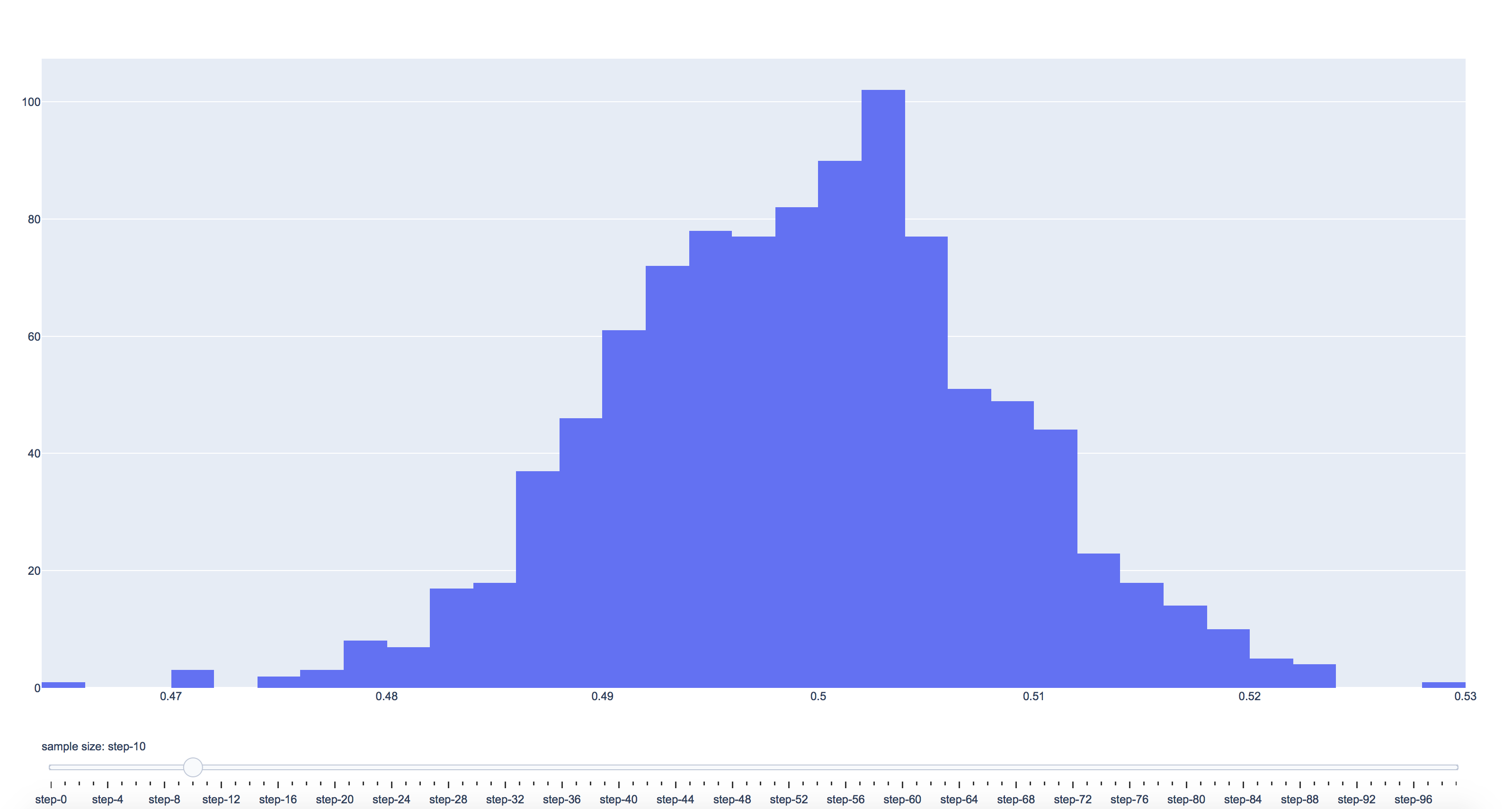
You can change below line of code to any form of distribution(beta, exponential, lognormal, gamma, etc). You will find out the underlying distribution does not affect much. If the distribution is skewed, such as exponential distribution, you will need larger N to observe this situation. If the distribution is less skewed, such as uniform distribution, you will be able to see it approximate to normal even though N is not big enough

x = np.array([np.average(np.random.uniform(0,1,size= step)) for i in range(1,1001)])